Posts

8 Sep 2025

Layout algorithms for flexigrids

This post is a development journal entry for the fletcher package for Typst. Fletcher is a diagramming package that lets users place nodes (content) on a flexigrid.

Flexigrids are a cross between a table layout and a coordinate grid. Unlike tables, flexigrids allow fractional coordinates, and unlike Cartesian coordinates, flexigrids automatically grow to accommodate content.

This leads to some interesting puzzles in terms of the best layout algorithm for computing row and column sizes given a set of nodes and their coordinates.

17 Mar 2025

Expression Synth 🎶

Fullscreen version

15 Sep 2024

French verb conjugations quizzer

Practice conjugating French verbs in specific tenses and moods. By changing the menus and toggles, you can practice conjugating verbs, distinguishing tenses by how they sound or are written, or even your pronunciation.

Fullscreen version, source code

19 Aug 2023

Basic general relativity with Julia

Four years after I took general relativity, my professor asked me to send him an old animation I had made during his course showing parallel transport of vectors around a line of latitude on the sphere. Actually, I wasn’t the one who had made it (though I was flattered that he had thought so!)

The tool I reached for was Julia. To my delight, the whole thing was rather simple to make. This was the humble result:

24 Apr 2023

Defining Entropy with a Composition Law

The mathematical definition of entropy is often hard to motivate, coming across as rather mysterious. But it can be uniquely characterised with a very natural and pretty ‘composition law’, which anyone could come up with.

Theorem: The formula for information entropy

$$ H(𝒑) = -K \sum_{i} p_i \log_2 p_i $$

is the unique real-valued function of a finite probability distribution $𝒑$ which:

is continuous with respect to $𝒑$,
obeys the Composition Law,
increases for uniform distributions $𝒑 = (\frac1n, ..., \frac1n)$ as the width $n$ increases,
has some fixed value $K$ for a fair coin toss $𝒑 = (\frac12, \frac12)$.

The last assumption is merely a choice of units — without it, the function is defined up to an overall scaling factor.

9 Jan 2023

Daylight Hours: A spherical geometry problem

How many hours are there between sunrise and sunset? The Earth’s tilt makes this a fun geometry problem…

Hours of daylight at the solstice

Let $ε$ be the Earth’s tilt, or obliquity. This is the angle between Earth’s axis of rotation $N$ and the normal to Earth’s orbital plane around the sun, $O$. At first, let’s assume that the Earth tilts directly toward the sun (or directly away, for $ε < 0$). This direct alignment occurs twice a year, at the summer and winder solstices. We can consider seasons later; for now, assume we’re at summer solstice.

11 Nov 2022

Billiard geometry: Visually solving elastic collisions

Suppose two bodies with initial momentum vectors $𝒑_1$ and $𝒑_2$ collide, so that the final momenta are $𝒑_1'$ and $𝒑'_2$.

If no restrictions are placed on these four momentum vectors, then we can describe all kinds of collisions, including ones that violate momentum and energy conservation.

12 Mar 2022

Geometric Algebra for Special Relativity and Manifold Geometry · PDF

My master’s thesis in mathematical physics completed in March 2022 at Victoria University of Wellington.

The thesis centres around geometric algebra and its applications to special relativity.

Table of Contents

I. Geometric Algebra and Special Relativity

Introduction
Preliminary Theory
- Associative Algebras
- The Wedge Product: Multivectors
- The Metric: Length and Angle
The Geometric Algebra
- Construction and Overview
- Relations to Other Algebras
- Rotors and the Associated Lie Groups
- Higher Notions of Orthogonality
- More Graded Products
The Algebra of Spacetime
- The Space/Time Split
- The Invariant Bivector Decomposition
- Lorentz Conjugacy Classes
Composition of Rotors in terms of their Generators
- A Geometric BCHD Formula
- BCHD Composition in Spacetime
Calculus in Flat Geometries
- Differentiation of Fields
- Case Study: Maxwell’s Equations

II. Geometric Algebra and Special Relativity

6 Mar 2022

World Flags Quizzer

Learn world flags by getting quizzed!

Flags are chosen randomly weighted by the country’s population. Press Check or type enter to submit your answer, and type ? to show the flag’s country name. Flags you get right in one try are “memorized” and won’t be shown again.

Fullscreen version

19 Oct 2021

A Simple Example of a Connection With Torsion

While learning general relativity as an undergrad, I was uneasy with the idea of torsion of an affine connection. Familiar phrases like “torsion measures how a frame twists as it undergoes parallel transport” seemed too lofty to serve as a helpful mental model.

The following example is one which gave me an aha! moment.

A “rolling” connection on $ℝ^2$.

Consider a connection on the plane defined in such a way that a vector undergoing parallel transport rotates in the $xy$-plane in proportion to its motion along the $x$-direction. That is, define a connection so that the vector field defined by

16 Aug 2021

Timeline of Scientists

This is an interactive timeline of famous mathematicians and physicists throughout history. The data is pulled from Wikidata.

Showing scientists, in decreasing order of number of Wikidata entities named after them. Hold `alt` and scroll to zoom.

12 Jul 2021

Explicit Baker–Campbell–Hausdorff–Dynkin formula for Spacetime via Geometric Algebra · arχiv

In brief. In $≤4$ dimensions, there’s a simple formula for the bivector $σ_3$ in terms of bivectors $σ_1$ and $σ_2$ such that $e^{σ_1}e^{σ_2} = ±e^{σ_3}$.

Abstract. We present a compact Baker–Campbell–Hausdorff–Dynkin formula for the composition of Lorentz transformations $e^{σ_i}$ in the spin representation (a.k.a. Lorentz rotors) in terms of their generators $σ_i$:

$$ \ln(e^{σ_1}e^{σ_2}) = \tanh^{-1}\qty(\frac{ \tanh σ_1 + \tanh σ_2 + \frac12\qty[\tanh σ_1, \tanh σ_2] }{ 1 + \frac12\qty{\tanh σ_1, \tanh σ_2} }) $$

This formula is general to geometric algebras (a.k.a. real Clifford algebras) of dimension $≤ 4$, naturally generalising Rodrigues’ formula for rotations in $ℝ^3$. In particular, it applies to Lorentz rotors within the framework of Hestenes’ spacetime algebra, and provides an efficient method for composing Lorentz generators. Computer implementations are possible with a complex $2×2$ matrix representation realised by the Pauli spin matrices. The formula is applied to the composition of relativistic $3$-velocities yielding simple expressions for the resulting boost and the concomitant Wigner angle.

9 Jul 2021

Mathematical One-liners

This is a collection of succinct but wonderfully satisfying theorems. Leave a comment if you have a good one!

27 Dec 2020

Light installation for Gatherings Restaurant

A projected light show made for a multi-sensory dining experience at Gatherings restaurant.

Interactive fullscreen version.

Act 0: Arrival

Pet nat // sparkling white wine, honey, fielding, clover, shoreline, waipara champagne, popping.
Canapes, kina w potato, ricotta and seaweed tart // refined, interesting, saline, creamy green.

7 Nov 2020

An Overview of the Strong CP Problem and Axion Cosmology · PDF

Literature review supervised by Dr. Jenni Adams at the University of Canterbury.

I wanted to learn more about particle physics after my Bachelor’s, so a year of part-time study culminated in this literature review. I learned basic classical (and a little quantum) field theory, and read about the “strong $CP$ problem” of quantum chromodynamics and its solution via “axions”. The report is aimed at the mathematically-inclined graduate who is uninitiated in particle physics.

17 Mar 2020

The Many Faces of Stokes’ Theorem

{% assign project_url = site.github.url | append: “/projects/stokes-theorem” %}

The generalised Stokes theorem has the remarkably compact form

$$ \boxed{ \int_Ω \dd ω = \int_{∂Ω} ω } $$

where $Ω$ is a $k$-dimensional manifold with boundary $∂Ω$, and $ω$ is a $(k - 1)$-form on $Ω$.

While it may seem alien at first when expressed in full generality, you may recognise some of the many special cases of Stokes’ theorem, especially from vector calculus.

15 Dec 2019

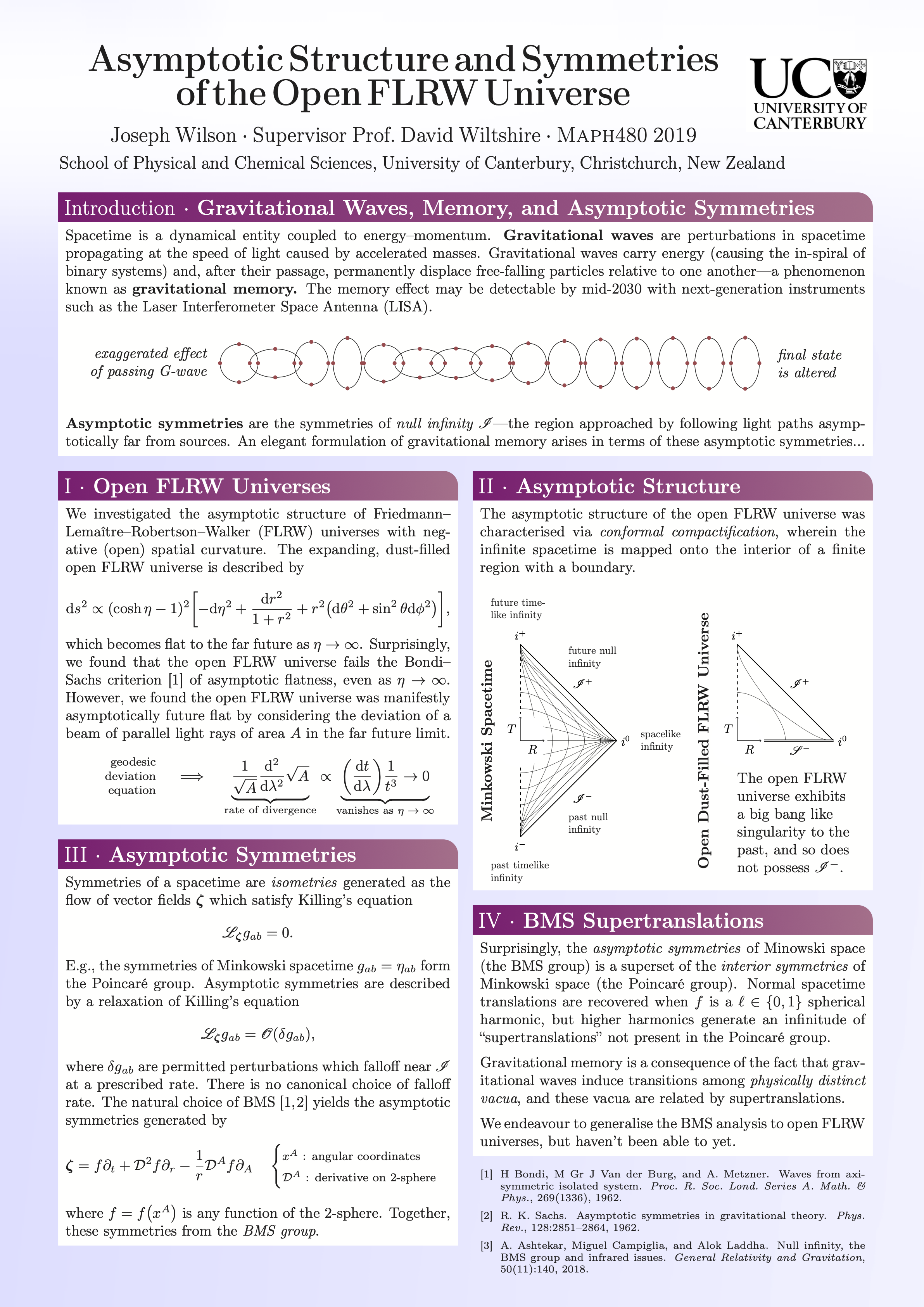
Asymptotic Structure and Symmetries of FLRW Universes · PDF

Honours project supervised by Prof. David Wiltshire at the University of Canterbury.

There is a fascinating relationship between the asymptotic symmetries of spacetime and gravitational waves and memory, sometimes referred to as The Infrared Triangle. We investigated the asymptotic structures of simple cosmological spacetimes, extending the usual analysis for flat spacetime.

You can find the full report (PDF) and also the poster (PDF).

15 Feb 2019

Computing Crystal Band Structures with CP2K · PDF

Summer project about the theory behind numerical computation of the semiconductor band structure of crystals using the open source software CP2K. Full PDF.

11 Sep 2018

Van Gogh's Starry Night as a phase portrait

The Dynamical Systems course I took had a competition to invent a dynamical system with the most creative phase portrait.

Here’s my entry: the Starry Night system.

# Scalar part
s := (-2*(y/2 - 1)^2 + θ((x - 4.63)^2 + (y - 167/50)^2 - 1/25)*θ(-(x - 91/20)^2 - (y - 82/25)^2 + 49/625) - 3*θ(x/50 - y + sin(15*x + 1)/10 + 22/25)/10 - 4*θ(2*x/25 - y + 117*sin(29*x/5 + 1.3)/1000 + 49/50)/5 + 4*θ(19*x/100 - y + 31*sin(17*x/5 + 84/25)/200 + .77)/5 + 5/2 + 27*exp(-(100*(x - .19)^2 + 100*(y - 43/20)^2)^2)/10 + 3*exp(-(100*(x - 1/2)^2/7 + 100*(y - 19/5)^2/7)^2) + 27*exp(-(500*(x - 31/50)^2/11 + 500*(y - 2.07)^2/11)^2)/10 + 2*exp(-(50*(x - 57/50)^2 + 50*(y - 191/50)^2)^2) + 4*exp(-(20*(x - 29/25)^2 + 20*(y - 82/25)^2)^2) + 3*exp(-(50*(x - 8/5)^2 + 50*(y - 67/25)^2)^2) + 3*exp(-(200*(x - 1.69)^2/7 + 200*(y - 19/5)^2/7)^2)/2 + 2*exp(-(25*(x - 1.73)^2/3 + 25*(y - 1.9)^2/3)^2) + 3*exp(-(250*(x - 2)^2/3 + 250*(y - 93/25)^2/3)^2) + exp(-(5*(x - 5/2)^2/3 + 5*(y - 13/5)^2/3)^2) + 2*exp(-(250*(x - 76/25)^2/11 + 250*(y - 3.63)^2/11)^2) + exp(-(20*(x - 69/20)^2/3 + 20*(y - 2.1)^2/3)^2) + 2*exp(-(250*(x - 3.51)^2/11 + 250*(y - 76/25)^2/11)^2) + 27*exp(-(5*(x - 91/20)^2/2 + 5*(y - 169/50)^2/2)^2)/10)*θ(y + 7*abs(-x + 17*y*sin(13*y/5 + 4.33)/250 + .91) - 2.7)*θ(y + 10*abs(x + (-17*y/250 + 21/125)*sin(5*y/2 + 1.7) - 29/25) - 47/20)*θ(y + 10*abs(x + (-17*y/250 + 21/125)*sin(31*y/5 - 12/5) - 37/40) - 73/20)*θ(y + 121*abs(x + (-17*y/250 + 21/125)*sin(157*y/25 + 24/5) - 1.49)/50 - 1.63)*θ(y + 64*abs(x + (-17*y/250 + 21/125)*sin(79*y/10 + 3) - 2)/25 - .97)

# Vector part, x-component
v_x := (((((y - 82/25)*θ(-(x - 91/20)^2 - (y - 82/25)^2 + 2/5) + ((y - 43/20)*θ(-(x - .19)^2 - (y - 43/20)^2 + .01) + ((y - 2.07)*θ(-(x - 31/50)^2 - (y - 2.07)^2 + 11/500) + ((y - 76/25)*θ(-(x - 3.51)^2 - (y - 76/25)^2 + 11/250) + ((y - 3.63)*θ(-(x - 76/25)^2 - (y - 3.63)^2 + 11/250) + ((y - 93/25)*θ(-(x - 2)^2 - (y - 93/25)^2 + 3/250) + ((y - 19/5)*θ(-(x - 1.69)^2 - (y - 19/5)^2 + 7/200) + ((y - 191/50)*θ(-(x - 57/50)^2 - (y - 191/50)^2 + 1/50) + ((y - 19/5)*θ(-(x - 1/2)^2 - (y - 19/5)^2 + .07) + ((y - 82/25)*θ(-(x - 29/25)^2 - (y - 82/25)^2 + 1/20) + ((y - 67/25)*θ(-(x - 8/5)^2 - (y - 67/25)^2 + 1/50) + ((y - 1.9)*θ(-(x - 1.73)^2 - (y - 1.9)^2 + 3/25) + (-θ(-(x - 1.73)^2 - (y - 1.9)^2 + 3/25) + 1)*((2*x/5 - y + 77/25)/((x - .3)^2/4 + (y - 16/5)^2/4)^3 + (-2*x/5 + y - 41/25)/((x - 12/5)^2/4 + (y - 13/5)^2/4)^3 + (2*x/5 - y + 37/50)/((x - 17/5)^2 + (y - 2.1)^2)^3))*(-θ(-(x - 8/5)^2 - (y - 67/25)^2 + 1/50) + 1))*(-θ(-(x - 29/25)^2 - (y - 82/25)^2 + 1/20) + 1))*(-θ(-(x - 1/2)^2 - (y - 19/5)^2 + .07) + 1))*(-θ(-(x - 57/50)^2 - (y - 191/50)^2 + 1/50) + 1))*(-θ(-(x - 1.69)^2 - (y - 19/5)^2 + 7/200) + 1))*(-θ(-(x - 2)^2 - (y - 93/25)^2 + 3/250) + 1))*(-θ(-(x - 76/25)^2 - (y - 3.63)^2 + 11/250) + 1))*(-θ(-(x - 3.51)^2 - (y - 76/25)^2 + 11/250) + 1))*(-θ(-(x - 31/50)^2 - (y - 2.07)^2 + 11/500) + 1))*(-θ(-(x - .19)^2 - (y - 43/20)^2 + .01) + 1))*(-θ(-(x - 91/20)^2 - (y - 82/25)^2 + 2/5) + 1))*(-θ(19*x/100 - y + 31*sin(17*x/5 + 84/25)/200 + .77) + 1) + θ(19*x/100 - y + 31*sin(17*x/5 + 84/25)/200 + .77))*(-θ(2*x/25 - y + 117*sin(29*x/5 + 1.3)/1000 + 49/50) + 1) + θ(2*x/25 - y + 117*sin(29*x/5 + 1.3)/1000 + 49/50))*(-θ(x/50 - y + sin(15*x + 1)/10 + 22/25) + 1) + θ(x/50 - y + sin(15*x + 1)/10 + 22/25))*θ(y + 7*abs(-x + 17*y*sin(13*y/5 + 4.33)/250 + .91) - 2.7)*θ(y + 10*abs(x + (-17*y/250 + 21/125)*sin(5*y/2 + 1.7) - 29/25) - 47/20)*θ(y + 10*abs(x + (-17*y/250 + 21/125)*sin(31*y/5 - 12/5) - 37/40) - 73/20)*θ(y + 121*abs(x + (-17*y/250 + 21/125)*sin(157*y/25 + 24/5) - 1.49)/50 - 1.63)*θ(y + 64*abs(x + (-17*y/250 + 21/125)*sin(79*y/10 + 3) - 2)/25 - .97) + (-θ(y + 7*abs(-x + 17*y*sin(13*y/5 + 4.33)/250 + .91) - 2.7)*θ(y + 10*abs(x + (-17*y/250 + 21/125)*sin(5*y/2 + 1.7) - 29/25) - 47/20)*θ(y + 10*abs(x + (-17*y/250 + 21/125)*sin(31*y/5 - 12/5) - 37/40) - 73/20)*θ(y + 121*abs(x + (-17*y/250 + 21/125)*sin(157*y/25 + 24/5) - 1.49)/50 - 1.63)*θ(y + 64*abs(x + (-17*y/250 + 21/125)*sin(79*y/10 + 3) - 2)/25 - .97) + 1)*sin(8*x)*sin(6*y)

# Vector part, y-component
v_y := (y + 1/5)*(-θ(y + 7*abs(-x + 17*y*sin(13*y/5 + 4.33)/250 + .91) - 2.7)*θ(y + 10*abs(x + (-17*y/250 + 21/125)*sin(5*y/2 + 1.7) - 29/25) - 47/20)*θ(y + 10*abs(x + (-17*y/250 + 21/125)*sin(31*y/5 - 12/5) - 37/40) - 73/20)*θ(y + 121*abs(x + (-17*y/250 + 21/125)*sin(157*y/25 + 24/5) - 1.49)/50 - 1.63)*θ(y + 64*abs(x + (-17*y/250 + 21/125)*sin(79*y/10 + 3) - 2)/25 - .97) + 1) + (((((-x + 91/20)*θ(-(x - 91/20)^2 - (y - 82/25)^2 + 2/5) + ((-x + .19)*θ(-(x - .19)^2 - (y - 43/20)^2 + .01) + ((-x + 31/50)*θ(-(x - 31/50)^2 - (y - 2.07)^2 + 11/500) + ((-x + 3.51)*θ(-(x - 3.51)^2 - (y - 76/25)^2 + 11/250) + ((-x + 76/25)*θ(-(x - 76/25)^2 - (y - 3.63)^2 + 11/250) + ((-x + 2)*θ(-(x - 2)^2 - (y - 93/25)^2 + 3/250) + ((-x + 1.69)*θ(-(x - 1.69)^2 - (y - 19/5)^2 + 7/200) + ((-x + 57/50)*θ(-(x - 57/50)^2 - (y - 191/50)^2 + 1/50) + ((-x + 1/2)*θ(-(x - 1/2)^2 - (y - 19/5)^2 + .07) + ((-x + 29/25)*θ(-(x - 29/25)^2 - (y - 82/25)^2 + 1/20) + ((-x + 8/5)*θ(-(x - 8/5)^2 - (y - 67/25)^2 + 1/50) + ((-x + 1.73)*θ(-(x - 1.73)^2 - (y - 1.9)^2 + 3/25) + (-θ(-(x - 1.73)^2 - (y - 1.9)^2 + 3/25) + 1)*((7*x/10 + 7*y/25 - 553/500)/((x - .3)^2/4 + (y - 16/5)^2/4)^3 + (-7*x/10 - 7*y/25 + 301/125)/((x - 12/5)^2/4 + (y - 13/5)^2/4)^3 + (7*x/10 + 7*y/25 - 371/125)/((x - 17/5)^2 + (y - 2.1)^2)^3))*(-θ(-(x - 8/5)^2 - (y - 67/25)^2 + 1/50) + 1))*(-θ(-(x - 29/25)^2 - (y - 82/25)^2 + 1/20) + 1))*(-θ(-(x - 1/2)^2 - (y - 19/5)^2 + .07) + 1))*(-θ(-(x - 57/50)^2 - (y - 191/50)^2 + 1/50) + 1))*(-θ(-(x - 1.69)^2 - (y - 19/5)^2 + 7/200) + 1))*(-θ(-(x - 2)^2 - (y - 93/25)^2 + 3/250) + 1))*(-θ(-(x - 76/25)^2 - (y - 3.63)^2 + 11/250) + 1))*(-θ(-(x - 3.51)^2 - (y - 76/25)^2 + 11/250) + 1))*(-θ(-(x - 31/50)^2 - (y - 2.07)^2 + 11/500) + 1))*(-θ(-(x - .19)^2 - (y - 43/20)^2 + .01) + 1))*(-θ(-(x - 91/20)^2 - (y - 82/25)^2 + 2/5) + 1))*(-θ(19*x/100 - y + 31*sin(17*x/5 + 84/25)/200 + .77) + 1) + (527*cos(17*x/5 + 84/25)/1000 + .19)*θ(19*x/100 - y + 31*sin(17*x/5 + 84/25)/200 + .77))*(-θ(2*x/25 - y + 117*sin(29*x/5 + 1.3)/1000 + 49/50) + 1) + (3393*cos(29*x/5 + 1.3)/5000 + 2/25)*θ(2*x/25 - y + 117*sin(29*x/5 + 1.3)/1000 + 49/50))*(-θ(x/50 - y + sin(15*x + 1)/10 + 22/25) + 1) + (3*cos(15*x + 1)/2 + 1/50)*θ(x/50 - y + sin(15*x + 1)/10 + 22/25))*θ(y + 7*abs(-x + 17*y*sin(13*y/5 + 4.33)/250 + .91) - 2.7)*θ(y + 10*abs(x + (-17*y/250 + 21/125)*sin(5*y/2 + 1.7) - 29/25) - 47/20)*θ(y + 10*abs(x + (-17*y/250 + 21/125)*sin(31*y/5 - 12/5) - 37/40) - 73/20)*θ(y + 121*abs(x + (-17*y/250 + 21/125)*sin(157*y/25 + 24/5) - 1.49)/50 - 1.63)*θ(y + 64*abs(x + (-17*y/250 + 21/125)*sin(79*y/10 + 3) - 2)/25 - .97)

# Normalisation of vector part
norm := sqrt(v_x^2 + v_y^2)

# Final system
dx/dt := s*v_x/norm
dy/dt := s*v_y/norm

The equations were not written by hand, of course, but generated by linearly combining simpler subsystems in an object oriented manner with Python.

15 Feb 2018

Visualising the Freudenreich 1998 Model of the Galactic Bar and Disk · PDF

Cosmology summer project in which we reproduced an empirical model of our galaxy’s centre and wrote code to visualise it. Full PDF.