The mathematical definition of entropy is often hard to motivate, coming across as rather mysterious. But it can be uniquely characterised with a very natural and pretty ‘composition law’, which anyone could come up with.
Theorem: The formula for information entropy
\[H(𝒑) = -K \sum_{i} p_i \log_2 p_i\]is the unique real-valued function of a finite probability distribution \(𝒑\) which:
- is continuous with respect to \(𝒑\),
- obeys the Composition Law,
- increases for uniform distributions \(𝒑 = (\frac1n, ..., \frac1n)\) as the width \(n\) increases,
- has some fixed value \(K\) for a fair coin toss \(𝒑 = (\frac12, \frac12)\).
The last assumption is merely a choice of units — without it, the function is defined up to an overall scaling factor.
Motivating the Composition Law
If we wanted to define the ‘uncertainty’ associated with a distribution, what properties should our measure have?
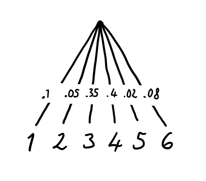
You can picture a finite probability distribution as a decision tree with weighted branches:
The same distribution can also be expressed by dividing the decision tree up into a composition of sub-trees:
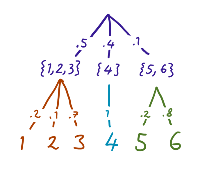
Notice that each final outcome still has the same overall probability — all we’ve done is add an extra ‘step’ in the random process.
Since these two pictures represent the same scenario, we want our uncertainty measure to be the same for both. But the second picture has many parts. How do you measure the total uncertainty? By taking a weighted sum of the uncertainties of each sub-tree.
Why a weighted sum? Consider what should happen when one of the branches’ probabilities goes to zero: the total uncertainty should not include the uncertainty of the sub-tree under that branch, since it is certain that its outcomes won’t happen.
For example, the probability of \(\{5, 6\}\) is \(.1\) in the picture, so the total uncertainty contains only a small contribution from the green sub-tree.
Expressing this mathematically, the uncertainty measure \(H\) should satisfy

where the left hand side is the uncertainty of the distribution in the first picture, and the right hand side is the total uncertainty in the second picture.
Note that the probabilities on each branch are still important, but are just too small to draw.
Formally
Now we can codify this composition law more formally. Let
\[\begin{aligned} 𝒑: Ω &→ [0, 1] \\ i &↦ p_i \end{aligned}\]be a finite probability distribution which is normalised so that \(\sum_{i ∈ Ω} p_i = 1\). Let \(\sim\) be some equivalence relation on the set of outcomes, \(Ω\). Define the quotient distribution
\[\begin{aligned} 𝒑/{\sim}: Ω/{\sim} &→ [0, 1] \\ [i] &↦ \textstyle\sum_{j \sim i} p_j \end{aligned}\]where \([i]\) is the equivalence class of \(i\). This corresponds to taking a distribution and binning the outcomes. Also define the restricted distributions
\[\begin{aligned} 𝒑|_{[i]} : [i] &→ [0, 1] \\ j &↦ \frac{p_j}{\sum_{k \sim j} p_k} \end{aligned}\]which correspond to keeping only a subset of outcomes and renormalising the probabilities.
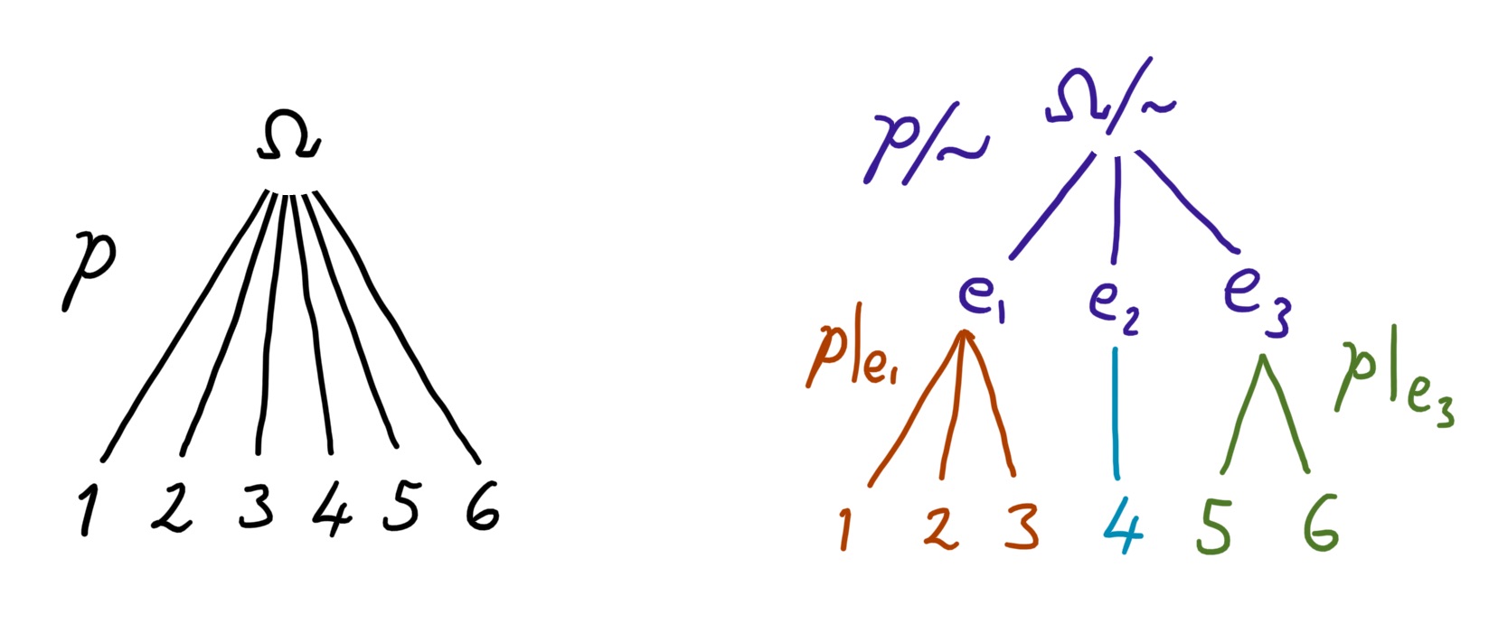
These fit into the example above where \(Ω = \{1, ..., 6\}\) like so:
Expressed in this language, the composition law is
\[H(𝒑) = H(𝒑/{\sim}) + \sum_{e ∈ Ω/{\sim}} (𝒑/{\sim})(e) \, H(𝒑|_e)\]where \((𝒑/{\sim})(e) = \sum_{i ∈ e} p_i\).
Proof of Uniqueness
We will prove that any ‘uncertainty’ function \(H(𝒑) ≡ H(p_1, ..., p_n)\) satisfying
- continuity
- the composition law
- the property that \(H(\frac1n, …, \frac1n)\) increases with \(n\)
must be equal to the Shannon entropy
\[H(𝒑) = -K \sum_{i} p_i \log_2 p_i\]where \(K = H(\frac12, \frac12)\). The proof is in three steps, one for each property above:
- Show that \(H(𝒑)\) is uniquely defined for all distributions \(𝒑\) if it is known for all rational distributions \(𝒒 ∈ ℚ^n\).
-
Show that \(H(𝒒)\) is uniquely defined for all rational distributions \(𝒒\) if the entropy of the uniform distribution
\[U(n) ≔ H(\underbrace{\textstyle\frac1n, ..., \frac1n}_n)\]is known for all \(n\).
- Show that \(U(n)\) is uniquely defined for all \(n\) if we fix \(U(2) = K\).
Step 1.
This follows by the assumption of continuity. If \(𝒑 ∈ ℝ^n\) is the limit a sequence of rational distributions \(𝒒_i ∈ ℚ^n\), then by continuity \(H(𝒑) = \lim_i H(𝒒_i)\).
Step 2.
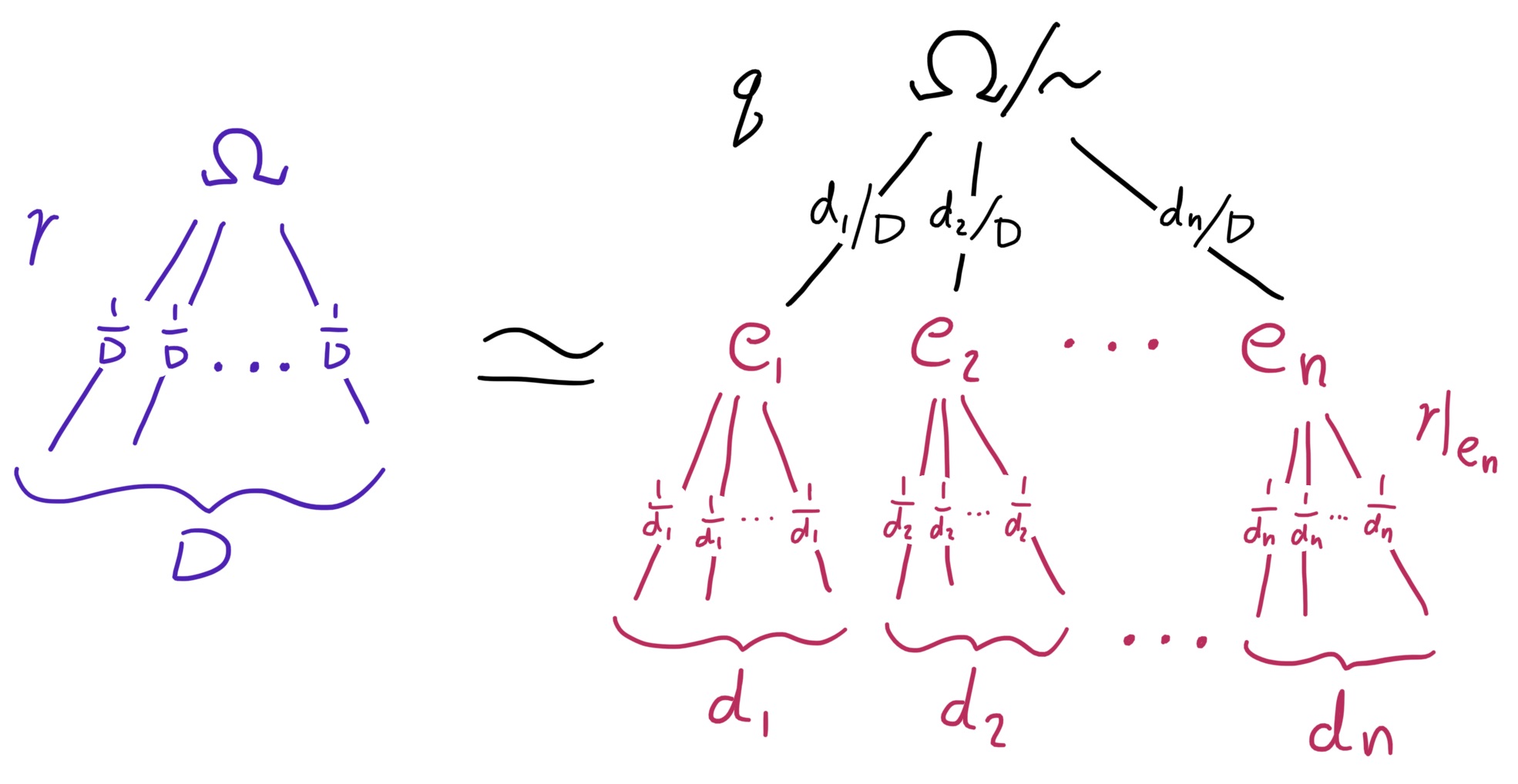
Let \(𝒒 ∈ ℚ^n\) be a rational distribution, and let \(D\) be the lowest common denominator of all the probabilities \(q_i\), so that
\[𝒒 = (d_1/D, d_2/D, ..., d_n/D)\]where \(d_i\) are non-negative integers. Now consider the set \(Ω = \{1, 2, ..., D\}\), and let \(𝒓(i) ≔ 1/D\) be the uniform distribution on \(Ω\). Define an equivalence relation \(\sim\) which partitions \(Ω\) into \(n\) different sets \(\{e_1, e_2, ..., e_n\}\), where the \(i\)th set contains \(d_i\) elements. The size of the \(i\)th equivalence group, as a fraction of the whole, is given by \(|e_i|/|Ω| = d_i/D = q_i\), and we have \(𝒓/{\sim} = 𝒒\) by construction.
From the composition law, we have
\[\begin{aligned} H(𝒓) &= H(𝒓/{\sim}) + \sum_{i = 1}^n \frac{d_i}D \, H(𝒓|_{e_i}) \\ U(D) &= H(𝒒) + \sum_{i=1}^n \frac{d_i}D \, U(d_i) \end{aligned}\]since \(H(𝒓) = U(D)\) and \(H(𝒓|_{e_i}) = U(d_i)\). This shows that \(H(𝒒)\) is uniquely defined if \(U(n)\) is known for all \(n\).
Step 3.
We will now show that \(U(n)\) is uniquely defined by \(U(2)\) by showing that the only possible functions are
\[U(n) = K\log_2 n\]where \(K\) is a free parameter.
Consider a uniform distribution \(r\) on \(\{1, 2, ..., nm\}\) partitioned by \(\sim\) into \(n\) groups of \(m\), so that the \(i\)th equivalence class is \([ni] = \{ni, ni + 1, ni + m - 1\}\). Writing down the composition law for this partition yields
\[\begin{aligned} H(𝒓) &= H(𝒓/{\sim}) + \sum_{i = 1}^n \frac1n H(𝒓|_{[ni]}) \\ U(nm) &= U(n) + \sum_{i = 1}^n \frac1n U(m) \end{aligned}\]and hence \(U(nm) = U(n) + U(m)\). The only increasing functions \(U(n)\) satisfying this property are multiples of \(\log n\). By choosing \(U(2) ≔ K\), we fix \(U(n) = K\log_2 n\).
This completes the proof!
In summary, under the three assumptions, knowing \(U(2) ≡ H(\frac12, \frac12)\) is enough to uniquely define \(U(n)\) for all \(n\), which is in turn enough to uniquely define \(H(𝒒)\) for all rational distributions \(𝒒\), which is enough to define \(H\) completely.